I’ve spent 14 years on the IBM mainframes. It was and still is an amazing, exotic technology even most IT tech people will never get to touch in their lives. The mainframes may look intimidating, but with a bit of abstraction, aren’t so different from Linux. This complete illustrated tutorial guides newcomers to the z/OS step-by-step using Linux analogies.

Learn how to connect using “mainframe’s PuTTY” the qws3270, create files using “mainframe’s Midnight Commander” the ISPF/PDF, edit files using “mainframe’s VIM” the ISPFEDIT, scripting using “mainframe’s bash” the JCL, and controlling it all using “mainframe’s task manager” the SDSF/Sysview.

Connecting to Mainframe: the 3270 terminal emulator

Mainframes are servers located in a datacenter far, far away. So exactly like you would use PuTTY terminal emulator to connect to a remote Linux server’s console over the internet, you need a terminal emulator for connecting to the mainframe.

These emulators are usually called “something3270”, which is a hint to the ancient mainframe console resolution – 32 lines of 70 characters. But don’t you worry, today, you can have as many lines and columns as you want!

Probably the most ubiquitous emulator is the QWS3270 from the Jolly Giant Software. There are others, even FOSS emulators like the x3270 available on Linux, and you can even connect to mainframes from Apple iOS today. But I always worked with QWS3270 as far as I can recall.

When you first start the 3270 terminal, it will ask you to provide connection information – just like PuTTY. Off course you have no idea, so you have to ask around. Remember to also ask about the ports and SSL – that’s in the Security tab.

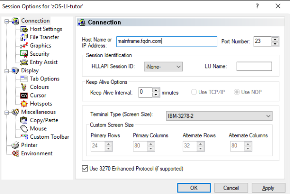
Besides the connection, the important setup here is the terminal size. If you keep the default Terminal Type of IBM-3278, then you’d be limited to the low screen resolution of 32 rows x 72 characters. Keep it for the first connection and as a backup, but once you get the feel for it, create a new profile using IBM-DYNAMIC.

With IBM-DYNAMIC, you can customize any resolution you want… With two caveats. The aspect ratio has to match the defaults, or some interactive GUI elements won’t scale properly and you will get a mess instead of UI. And initially, you won’t see any effect – you’d have to enable the DYNAMIC terminal sizing on the remote, z/OS side as well.

First connection (or when something fails): the TSO red screen

After you connect, you will be usually greeted by a company-specific console-GUI front end for selecting one of many mainframe virtual systems available. Because IBM was doing Virtual Machines before it was cool. Past that, and possibly past one more login screen, you will either be greeted with console-GUI, or with a screen of red text:

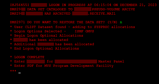
The red screen is the TSO, the basic layer of z/OS. You can think of it as of the Linux Shell on a console-only Linux servers. You can issue text commands, documented in the IBM TSO User guide and Command reference (available here in PDF, just download all these things when you start with zOS.) You can also use the IBM’s TSO commands Cheat-Sheet, but it won’t be of much use without searching the syntax anyway.

Fortunately, you will not be using TSO much, as there are easier alternatives.

Just if you press F3, which serves as “back” key on the z/OS, too much, you can find yourself here.

If you write PDF (or, on other systems, ISPF or other custom command), you switch to the “terminal GUI”.

ISPF / PDF: the terminal screen GUI panels

Do you remember the “console GUI applications”, like the Norton Commander on DOS or Midnight Commander on Linux, or the old Debian installer? The same is the foundation of working with the z/OS. ISPF is the name of the technology – you can code your own custom panels if you want.

Most companies use a heavily customized ISPF panels with some fancy ASCIIart graphics, but this is moreorless the IBM default:

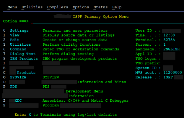
You can safely ignore most of it for starters, because only three of these menus are really important.

When you first connect to your session on z/OS, write

0

On the Options commandline and confirm with your submit key. What? Right, I forgot to tell you. Mainframes distinguish between “enter/newline” key, which just harmlessly jumps to the beginning of the next line… And between “enter/control” key, which submits a command or whatever. The reverse to the “enter/control” is the F3 key, which is like a “back/close” button.

Most mainframers set the right Control key as their submit key (in the terminal keyboard options):

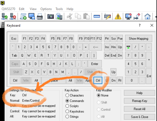
So, once more – write “0”, hit your right Ctrl, and you get the ISPF settings. The thing important for the beginners here is the Screen format:

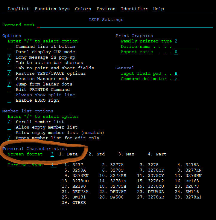
Because this is what you need to use the high screen resolution (err, character resolution?) offered by the IBM-DYNAMIC settings of your terminal emulator.

Overwrite the number on the value field with 3, press control/enter. Press “F3” to exit (in Mainframe lingo, it’s actually “PF3” – better get used to that). You’re once more on the main ISPF/PDF screen. So let’s get to business!

Crash course into Mainframe files and filesystem

As there are certain differences between files and folders/directories between Windows and Linux (eg. on Linux, directory is a file), even more profound differences are between LUW and Mainframe.

For starters, mainframers call their files “datasets”.

And you have these basic dataset types familiar from LUW (true mainframers will forgive me the heresy of making comparisons):

• Sequential dataset (PS) is like a normal LUW flat file. You can edit the contents in a text editor, etc.
• Library or Partitioned Dataset (PDS/PDSE) is like your LUW directory. It contains multiple files inside. Caveat: each PDS can only contain files, not recursive directories!
• PO (RECFM=U) is like your LUW binary executable file – the PE32 *.exe on Windows, or the Linux *.out. Same as on LUW, while you can open them in a text editor, you would just mess them up, so don’t.
• VSAM is like a database file – the closest LUW equivalent would be something like SQLite database file. It’s actually two files under one name – the database and it’s index. You cannot directly edit these, nor copy them over, without using special utilities. Don’t touch them for the time being, okay?

Then we need some mainframe knowledge on paths and filenames. Exactly like you would write “C:\home\someguy\somefile.txt” on Windows, or “/home/somegal/somefile.txt” on Linux, on Mainframe, you would write this instead:

This entire thing is called “Dataset Name”, or DSN.

Does it look familiar to the LUW paths? Then let me let you down a bit: Mainframe filesystem doesn’t have the hierarchical structure of folders within folders within root folders or C: drive of the LUW. Because mainframe “folders” cannot contain more folders, remember?

But for all practical terms and purposes, the periods work the same way as slashes or backslashes between folder and file names on LUW, so as a beginner, you can safely pretend it is the same.

These period-separated filenames are hence like a LUW path and at the same time nothing like a path. Also, each segment can only be 8 characters long, and they can be only finite number of them. They’re called high-, medium- and low-level qualifiers, and this is the IBM doc on them.

Now to the business. The menu “3” in the ISPF/PDF will offer you a list of interactive GUI utilities for making and handling these files (minus VSAM). Write “3” on the “Option ===>” command line and press your control key to see them:

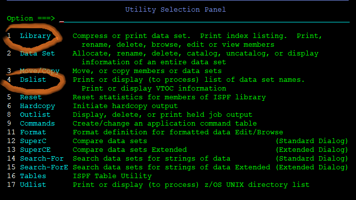
The only of these you will likely ever really need to use from the GUI is option 3.2 Data set, and 3.4 Dslist. Yes, you can use shortcuts like this on the command line to skip any number of screens!

The PDS.3.2 Data set utility – how to create a new empty file/folder on mainframe

Anyway, when you want to create (in mainframers lingo, “allocate”) a new file (“dataset”), you use the P.3.2 Dataset utility. When you open it, it is a two-stage process. On a first screen, you must not forget to write the letter “A” on the option commandline, and then write the intended dataset name onto the Name field down below:

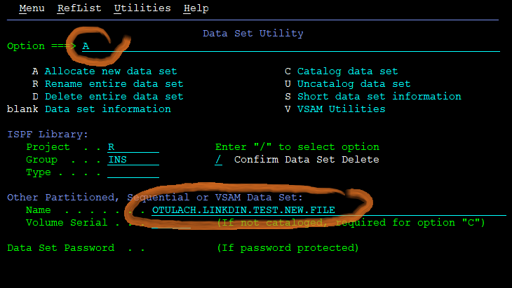
Then you can press enter (I mean Control) to proceed to the next screen, where you will determine the actual parameters of the file. And when I say “you will”, I mean “you must”:

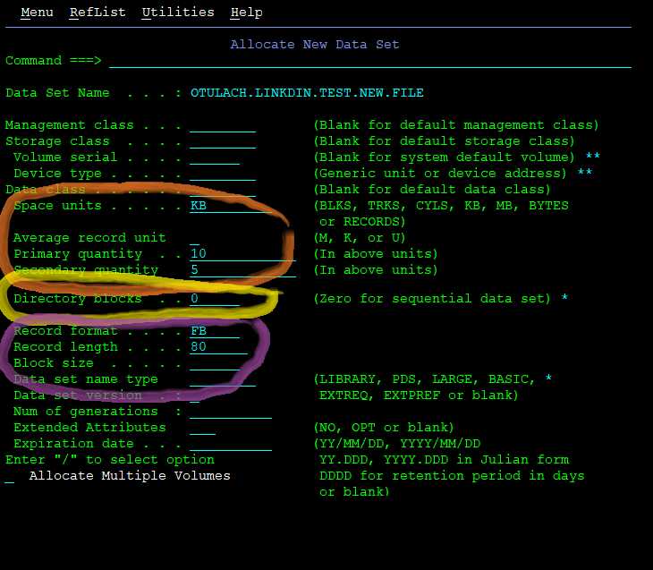
First the orange group on the screenshot. Remember how on LUW, your file size grows dynamically as you add contents? Well, forget about that. Mainframe is old technology, and for Sacred Reverse-Compatibility Reasons, you must still guess and allocate your maximal file size up-front! If your file exceeds it, too bad – you will get a write error.

But it’s at least a little bit smart. After you select your size units (LUW-friendly KB/MB or mainframe-native hard drive Blocks, Tracks and Cylinders), you get to choose actually two sizes:

• Primary size is how big the dataset will be when you create it.
• Secondary size is by how much the dataset will grow when you completely fill the previous size – at most 16× (or, for the new “extended” dataset types, up to 123×)

This predefined growth is called “extent”.

Then, super-important stuff – Directory blocks (yellow group). This is how you chose between creating a file or a folder! Directory blocks is like an index file of the directory’s file lists. This number determines how many files can the Library/PDS contain. If you set it to 0, you’re creating normal text dataset. Anything more – a directory.

And finally, the physical characteristics. Normal text datasets are written in records – fixed line lengths then blocked together for performance reasons. The Record length (abbreviated LRECL for Logical RECord Length) is the maximal allowed length of any line in your file, so choose it wisely. There are some informal standard lengths – 80 and 82 for JCL scripts, 133 and 137 for output files, and so on. But you can make a length of your choosing – and then bear the consequences.

But how does Record length impact folders? Easy – the LRECL you set for the folder becomes the maximal LRECL for any and all files inside that folder. So choose double-wisely.

If you are clueless what parameters to write in, there is a trick. If you write some existing dataset on the first screen of the 3.2 Dataset Utility, and then press control/enter on the commandline WITHOUT specifying any of the options, you display the information about the existing file:

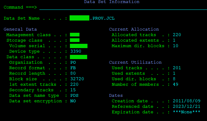
And wait for it… Now if you press PF3 to go back, you write a new dataset name, and use the “A” to allocate option and press enter again… All those parameters of the old reference file will be copied for you to the new file’s parameters!

But don’t worry, you will almost never use this P.3.2 Dataset utility after some while. Instead, you would be using

The PDS.3.4 Dslist utility: like your Windows Explorer, only hardcore

This utility is how you copy and delete both files and folders (libraries), and how you list, browse and edit files (sequential datasets).

On the first screen, you write the dataset name and press control/enter to begin:

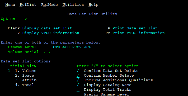
If you write the exact DSN, you will only get that single file or folder – like with Linux “ls -l” command, only interactive.

But like with Linux ls, you can use wildcards. And you can use them at any level!

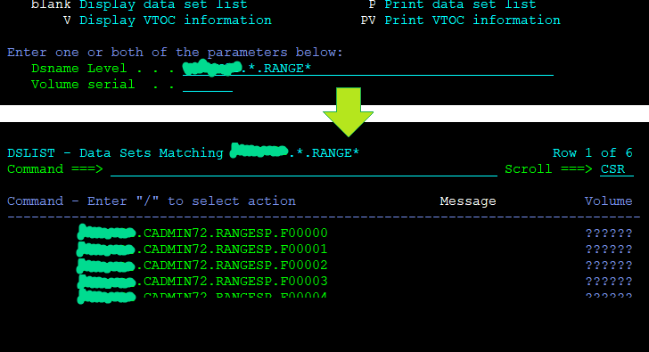
That brings us to the second screen. When you get the List of Datasets, you can write a letter to the left and press control/enter to execute.

• command C would trigger a Copy Dataset dialog
• command D would delete given file/folder
• command B would browse the file in read-only mode, or browse the folder’s members
• commands V or E would open the file in the ISPFVIEW and ISPFEDIT utility to advanced-view it with HEX and stuff, resp. to edit it

Let’s talk about this viewing and editing more.

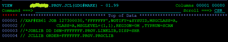
ISPFVIEW and ISPFEDIT – like a mainframe’s VIM, but more friendly

By default, the view/edit opens in vanilla mode:

But ISPFVIEW/EDIT is superbly powerful tool, with not one, but two control interfaces:

• you can issue text commands in the Command line
• you can issue line commands in the line numbers section on the left

Eg. say you want to see the HEX code of the contents. Either you can write HEX on the commandline and apply it to all (write HEX OFF to revert):

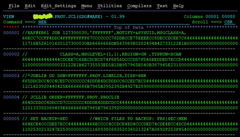
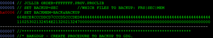
But if you feel that is an overkill, you can write HX to show hex of the exact line you’re interested in!

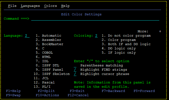
Oh, do you want syntax highlighting? Just write HILITE ON on the command line:

Either ISPFVIEW will guess what language it is, or it will ask you:

Want to do search-and-replace? Just issue command

c stringFrom stringTo all

Want to find something? Issue

f needleString

Want to scroll to a particular line number? Issue

l 1234

Want to copy or cut a line and move it somewhere? Use the line commands to M-ove that line A-fter or B-efore other line:

Want to repeat a line 12x? Just write

r 12

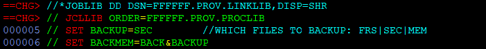
Want to repeat whole blocks? Or copy it? Use block commands RR or CC:

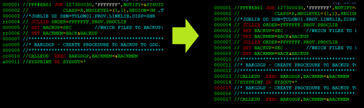
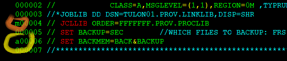
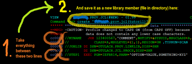
And finally, combinations. Eg. to cut/copy a portion (or entirety) of one file into another file, just combine the Line Block commands “CC-CC” to select lines to be copied/cut, and then Commandline command “cut” or “copy” to put it into another file (if you don’t specify round brackets) or library/directory (if you do specify round brackets and library member name, a.k.a. filename inside folder):

This is just a small demo what ISPFEDIT and ISPFVIEW can do. Some mainframers used to use their LUW equivalents even outside Mainframe. But that was before VSCode 🙂

Now you can use all that knowledge to write your first JCL script – the very first piece of workload to run on the mainframe. I’ve covered JCL in part 1 of this tutorial here.

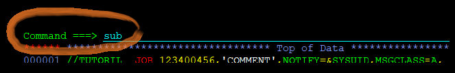
When you have completed your first JCL (and double-checked your Account code, CLASS and DD DISP statements not to be logged as security violator or deleting something you shouldn’t), you can schedule-run that JCL. In ISPFEDIT, just write “sub” (short for “submit”, both variants work) on the command line and hit control/enter:

SDSF or Sysview: the mainframe’s Task Managers

Now we know

1. how to login to mainframe and run the ISPF/PDF GUI,
2. how to create a dataset, eg. our personal JCL library “folder”
3. how to create, edit and save new files using ISPFEDIT
4. how to write and submit JCL jobs for execution

So the last task to become a junior mainframer is to check, debug, resubmit and otherwise control the actual execution, the run, of our jobs and programs!

Since we don’t get interactive Console window but instead schedule Jobs to Batch processing, we need to monitor our jobs, their success/failure and their results and logs inside the z/OS scheduling system itself. That system is called JES (for Job Execution System) and as always, check the IBM JES reference guide for more info. (Actually, you don’t need that as a junior.)

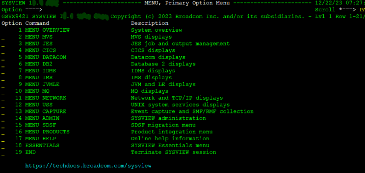
The mainframe equivalent of the Windows Task Manager is an IBM utility called SDSF – or it’s much better replacement, CA SYSVIEW (now part of Broadcom). It’s not that I’d like to praise my own feathers, I’ve never worked in the Sysview team – it’s just that having worked both with SDSF and Sysview, the latter is like light years better and more powerful!

But beware, I only ever used Sysview in a “SDSF backwards compatibility mode”, which is like SDSF but on steroids. Sysview has it’s own sysview-ish mode, which was always too overwhelming for me. There is a command to switch Sysview into the SDSF compatibility mode, which you just enter on Sysview command line; write it down just in case:

SET SDSFMIGRATE ON

The initial menu of SDSF resp. Sysview in SDSF-legacy mode looks like this. It is a crossroads to various monitors and task managers, which lists shortcuts to type on the command line:

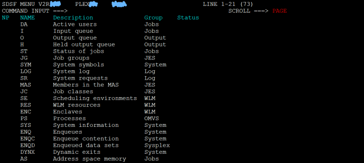
The task monitor is the “ST” option. Type ST into the commandline, control/enter, and you will see the list of JCl jobs running and finished. Er, all of the JCL jobs in the entire system:

That’s kinda too much, and it’s slow. So let’s filter on our own:

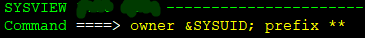
This sample command shows you four things:

• use owner keyword to filter on the username who has submitted the job
• use prefix, or pre, keyword to filter on the jobname
• you can use multiple filters separated by the ; separator
• you can use wildcards – single * for masking part of value, double ** for disabling the filter

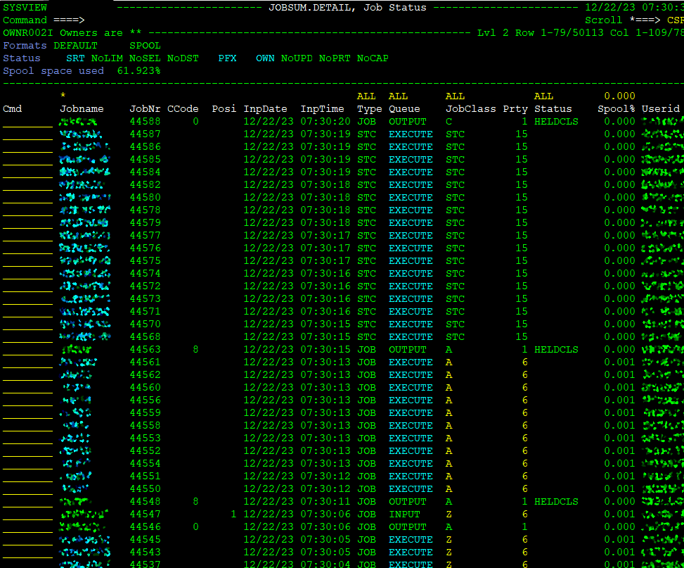
Once you do that, you can see the list of your JCL jobs you submitted – like the Linux PS command, but actually interactive and way more powerful.

One more important command is SORT. To intuitively sort jobs by their submit date and time in descending order, enter following command:

SORT STDATE,D,STTIME,D

The jobs displayed alter between phases INPUT (waiting in the queue for their turn), EXECUTE (running), OUTPUT (finished and logged) or HELD (paused or retained when done). And then some, but these are the basics:

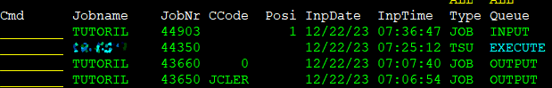
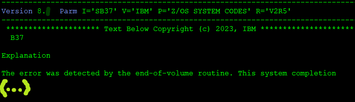
Notice that when the job has run, you get a Return Code (CCode). Alternatively, if it failed for syntax errors or pre-execute checks (eg. invalid dataset or so), you can get JCL error instead. And if something in the job failed horribly, you get ABEND, which is mainframe lingo for “brutal crash” like SIGSEV and others on Linux. Each Abend has it’s own code, and you will be diagnosing Abend codes often. Eg. SB037 Abend means that you messed up your dataset allocation and no new data can fit in.

---

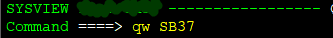
For this diagnostics, try to run the “qw SB37” on the command line. Some mainframe environments have bought and installed priceless amazing utility “Quick Reference“, which interactively displays the descriptions of error codes from all major vendors – IBM, CA/Broadcom, everyone! This saves eons of time spent searching the docs or the internet:

Just scroll down the item matching your interest (no, not BMC, the IBM System code) using the enter/newline, mark it “s” to select,

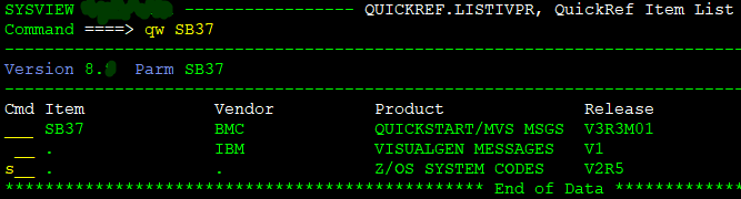
Press control/enter, and read on:

---

Back to SDSF/Sysview. See the little lines to the left of the job listings? That means it’s for line commands:

• S selects and prints output of the entire job – all the logs concatenated. You will drown in the log data. But sometimes you need this to find something hiding in other logfile than you’d expect!
• SE opens the printout of the entire job in ISPFEDIT, so that you can copypaste, vie HEX values etc., or copy it somewhere to a file.
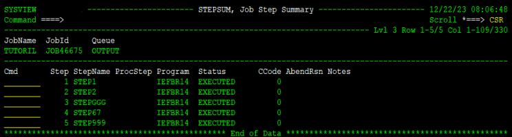
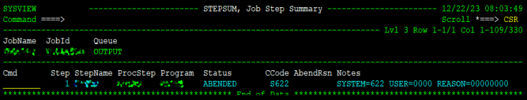
• SS allows you to select oputput/log of a single step – the one misbehaving. It displays a sub-menu with the list of that job’s steps, where you can further put S to see only that step’s logs. Ideal for diagnosing.
• L displays the various log files of that job. That is a different thing than the steps listing!
• SJ displays the JCL of the original job

This is SS opened for good job with multiple steps, versus for diagnosing ABEND-ed failed job:

Thus, the debug process:

1. Open SDSF or Sysview.
2. ST to see your jobs list.
3. S to print JCL error and find error message. Or L and select the JESYSMSG to see just JCL errors and logs. Or SS to see the steps listing. Find the last error message (you can use commandline ‘F errormesage PREV’ to search from the end back)
4. Diagnose using Quick Reference or PDF doc.
5. Go back to queue list, SJ to open the source code of the JCL in ISPFEDIT, fix what’s broken, re-submit.
6. Don’t forget to copy the fixed/debugged JCL from the JES queue / Sysview list back to the original dataset, so that you retain the fixed version and not the original bugged version!

Sysview can do much more. Monitor system resources (DASHBOARD OPERATOR instead of ST), list all hard drives in the system (DASD), list all volumes (akin to LUW logical partitions – VOL), monitor TCP/IP ports opened, etc. But this is enough for the basics.

That’s it

This is how my z/OS career started for me. My boss has shown me the login screen, ISPF P.2 and P.4 GUI screens to create files, and SDSF task manager – and thrown me to swim myself, equipped just with the MVS JCL Reference Manual. And I did, because that’s the bulk of it it.

So, congratulations. If you read this article and repeated the steps on-screen on a real mainframe, you are now a mainframer.